We’re going to pretend we have an actual product we need to improve. We will explore a dataset and try out different models like logistic regression, recurrent neural networks, and transformers, looking at how accurate they are, how they are going to improve the product, how fast they work, and whether they’re easy to debug and scale up.
You can read the full case study code on GitHub and see the analysis notebook with interactive charts in Jupyter Notebook Viewer.
Excited? Let’s get to it!
Imagine we own an E-commerce website. On this website, the seller can upload the descriptions of the items they want to sell. They also have to choose items’ categories manually which may slow them down.
Our task is to automate the choice of categories based on the item description. However, a wrongly automated choice is worse than no automatization, because a mistake might go unnoticed, which may lead to losses in sales. Therefore we might choose not to set an automated label if we’re not sure.
For this case study, we will use the Zenodo E-commerce text dataset, containing item descriptions and categories.
We will consider multiple model architectures below and it’s always a good practice to decide how to choose the best option before we start. How is this model going to impact our product? …our infrastructure?
Obviously, we will have a technical quality metric to compare various models offline. In this case, we have a multi-class classification task, so let’s use a balanced accuracy score, which handles imbalanced labels well.
Of course, the typical final stage of testing a candidate is AB testing – the online stage, which gives a better picture of how the customers are affected by the change. Usually, AB testing is more time-consuming than offline testing, therefore only the best candidates from the offline stage get tested. This is a case study, and we don’t have actual users, so we’re not going to cover AB testing.
What else should we consider before moving a candidate forward for AB-testing? What can we think about during the offline stage to save ourselves some online testing time and make sure that we’re really testing the best possible solution?
Balanced accuracy is great, but this score doesn’t answer the question “How exactly the model is going to impact the product?”. To find more product-oriented score we must understand how we are going to use the model.
In our setting, making a mistake is worse than giving no answer, because the seller will have to notice the mistake and change the category manually. An unnoticed mistake will decrease sales and make the seller’s user experience worse, we risk losing customers.
To avoid that, we’ll choose thresholds for the model’s score so that we only allow ourselves 1% of mistakes. The product-oriented metric can then be set as follows:
What percentage of items can we categorise automatically if our error tolerance is only 1%?
We’ll refer to this as Automatic categorisation percentage below when selecting the best model. Find the full threshold selection code here.
How long does it take a model to process one request?
This will roughly allow us to compare how much more resources we’ll have to maintain for a service to handle the task load if one model is selected over another.
When our product is going to grow, how easy will it be to manage the growth using given architecture?
By growth we might mean:
Will we have to rethink a model choice to handle the growth or a simple retrain will suffice?
How easy it will be to debug model’s errors while training and after deployment?
Model size matters if:
We’ll see later that both items above are not relevant, but it’s still worth considering briefly.
What are we working with? Let’s look at the data and see if it needs cleaning up!
The dataset contains 2 columns: item description and category, a total of 50.5k rows.
file_name = "ecommerceDataset.csv"
data = pd.read_csv(file_name, header=None)
data.columns = ["category", "description"]

print("Rows, cols:", data.shape)

# >>> Rows, cols: (50425, 2)
Each item is assigned 1 of the 4 categories available: Household, Books, Electronics or Clothing & Accessories. Here’s 1 item description example per category:
There’s just one empty value in the dataset, which we are going to remove.
print(data.info())

# <class 'pandas.core.frame.DataFrame'>
# RangeIndex: 50425 entries, 0 to 50424
# Data columns (total 2 columns):
#  #   Column       Non-Null Count  Dtype
# ---  ------       --------------  -----
#  0   category     50425 non-null  object
#  1   description  50424 non-null  object
# dtypes: object(2)
# memory usage: 788.0+ KB

data.dropna(inplace=True)
There are however quite a lot of duplicated descriptions. Luckily all duplicates belong to one category, so we can safely drop them.
repeated_messages = data \
    .groupby("description", as_index=False) \
    .agg(
        n_repeats=("category", "count"),
        n_unique_categories=("category", lambda x: len(np.unique(x)))
    )

repeated_messages = repeated_messages[repeated_messages["n_repeats"] > 1]

print(f"Count of repeated messages (unique): {repeated_messages.shape[0]}")
print(f"Total number: {repeated_messages['n_repeats'].sum()} out of {data.shape[0]}")

# >>> Count of repeated messages (unique): 13979
# >>> Total number: 36601 out of 50424
After removing the duplicates we’re left with 55% of the original dataset. The dataset is well-balanced.
data.drop_duplicates(inplace=True)
print(f"New dataset size: {data.shape}")
print(data["category"].value_counts())

# New dataset size: (27802, 2)
# Household                 10564
# Books                      6256
# Clothing & Accessories     5674
# Electronics                5308
# Name: category, dtype: int64
Note, that according to the dataset description,
The dataset has been scraped from Indian e-commerce platform.
The descriptions are not necessarily written in English. Some of them are written in Hindi or other languages using non-ASCII symbols or transliterated into the Latin alphabet, or use a mix of languages. Examples from Books category:
यू जी सी – नेट जूनियर रिसर्च फैलोशिप एवं सहायक प्रोफेसर योग्यता …Prarambhik Bhartiy ItihasHistory of NORTH INDIA/வட இந்திய வரலாறு/ …To evaluate the presence of non-English words in descriptions, let’s calculate 2 scores:
Word2Vec-300 trained on an English corpus.Using ASCII-score we learn that only 2.3% of the descriptions consist of more than 1% non-ASCII symbols.
def get_ascii_score(description):
    total_sym_cnt = 0
    ascii_sym_cnt = 0

    for sym in description:
        total_sym_cnt += 1
        if sym.isascii():
            ascii_sym_cnt += 1
    return ascii_sym_cnt / total_sym_cnt

data["ascii_score"] = data["description"].apply(get_ascii_score)
data[data["ascii_score"] < 0.99].shape[0] / data.shape[0]

# >>> 0.023
Valid English words score shows that only 1.5% of the descriptions have less than 70% of valid English words among ASCII words.
w2v_eng = gensim.models.KeyedVectors.load_word2vec_format(w2v_path, binary=True)

def get_valid_eng_score(description):
    description = re.sub("[^a-z \t]+", " ", description.lower())
    total_word_cnt = 0
    eng_word_cnt = 0

    for word in description.split():
        total_word_cnt += 1
        if word.lower() in w2v_eng:
            eng_word_cnt += 1
    return eng_word_cnt / total_word_cnt

data["eng_score"] = data["description"].apply(get_valid_eng_score)
data[data["eng_score"] < 0.7].shape[0] / data.shape[0]

# >>> 0.015
Therefore the majority of descriptions (around 96%) are in English or mostly in English. We can remove all other descriptions, but instead, let’s leave them as is and then see how each model handles them.
Let’s split our dataset into 3 groups:
from sklearn.model_selection import train_test_split

data_train, data_test = train_test_split(data, test_size=0.3)
data_test, data_eval = train_test_split(data_test, test_size=0.5)

data_train.shape, data_test.shape, data_eval.shape

# >>> ((19461, 3), (4170, 3), (4171, 3))
It’s helpful to do something straightforward and trivial at first to get a good baseline. As a baseline let’s create a bag of words structure based on the train dataset.
Let’s also limit the dictionary size to 100 words.
count_vectorizer = CountVectorizer(max_features=100, stop_words="english")

x_train_baseline = count_vectorizer.fit_transform(data_train["description"])
y_train_baseline = data_train["category"]

x_test_baseline = count_vectorizer.transform(data_test["description"])
y_test_baseline = data_test["category"]

x_train_baseline = x_train_baseline.toarray()
x_test_baseline = x_test_baseline.toarray()
I’m planning to use logistic regression as a model, so I need to normalize counter features before training.
ss = StandardScaler()
x_train_baseline = ss.fit_transform(x_train_baseline)
x_test_baseline = ss.transform(x_test_baseline)

lr = LogisticRegression()
lr.fit(x_train_baseline, y_train_baseline)

balanced_accuracy_score(y_test_baseline, lr.predict(x_test_baseline))
# >>> 0.752
Multi-class logistic regression showed 75.2% balanced accuracy. This is a great baseline!
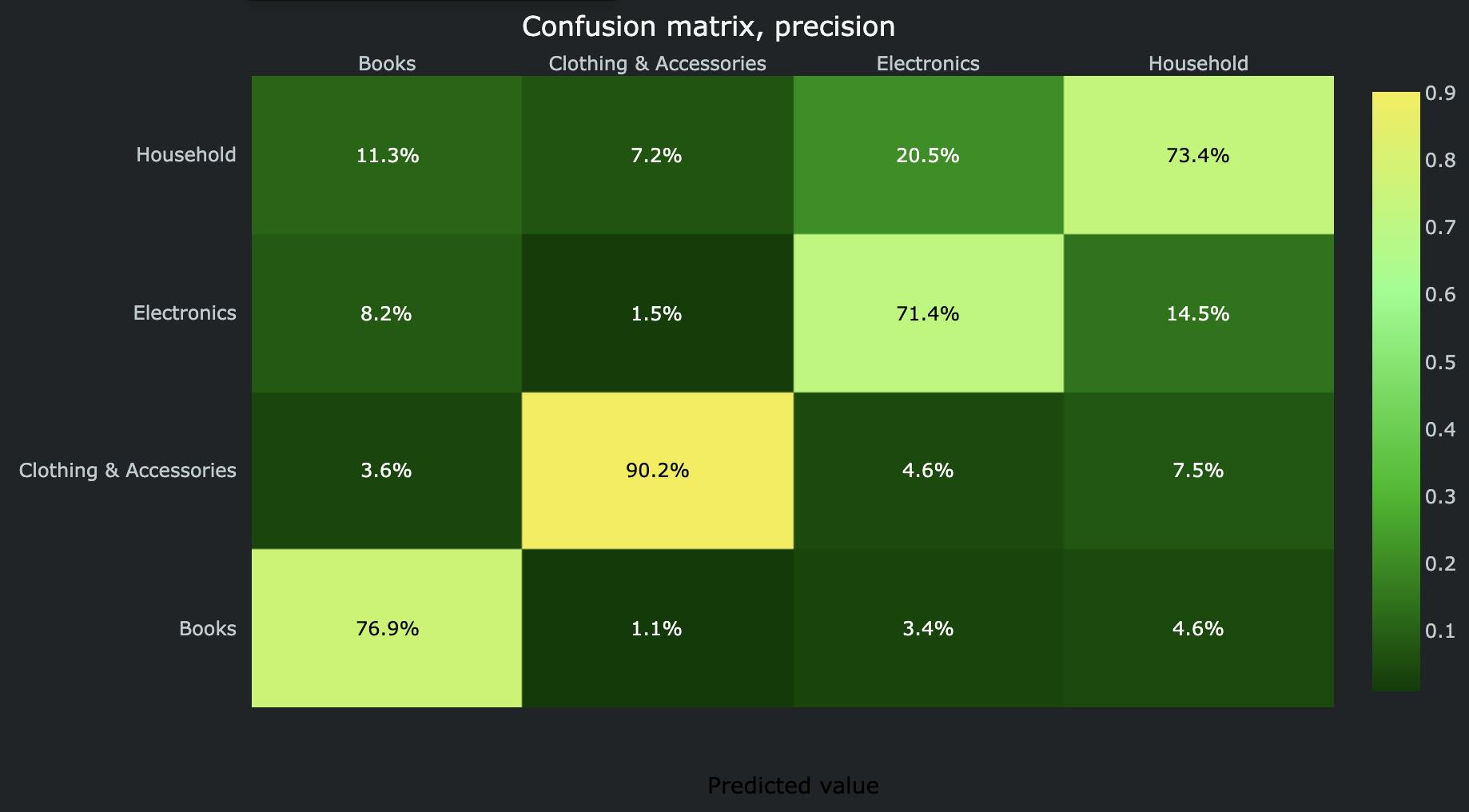
Although the overall classification quality is not great, the model can still give us some insights. Let’s look at the confusion matrix, normalized by the number of predicted labels. The X-axis denotes the predicted category, and the Y-axis – the real category. Looking at each column we can see the distribution of real categories when a certain category was predicted.
Confusion matrix for baseline solution.
For example, Electronics is frequently confused with Household. But even this simple model can capture Clothing & Accessories quite precisely.
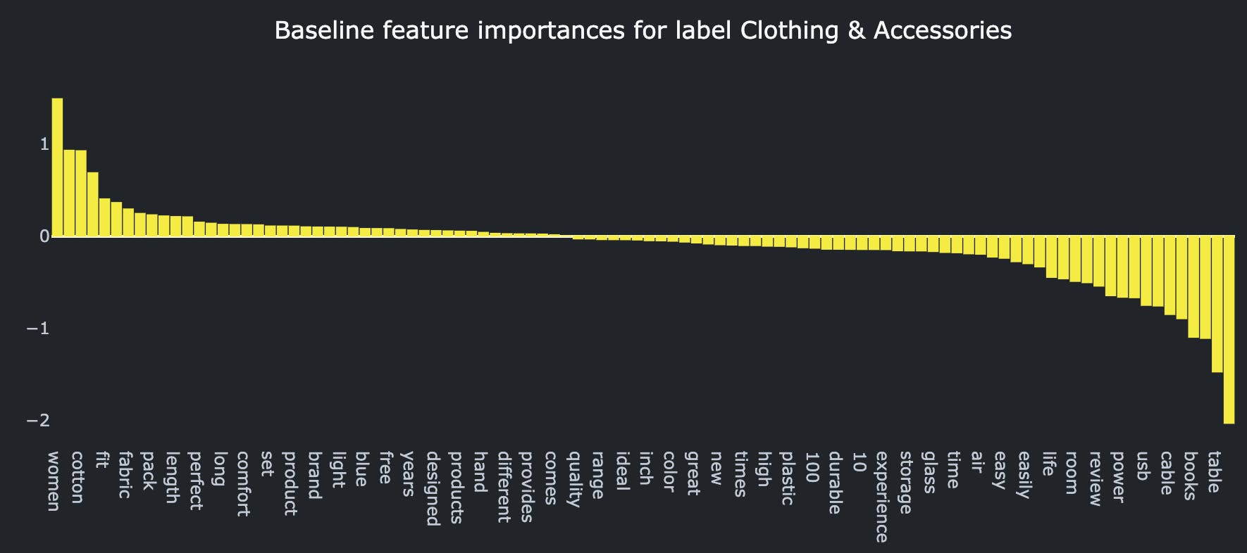
Here are feature importances when predicting Clothing & Accessories category:
Feature importances for baseline solution for label ‘Clothing & Accessories’
Top-6 most contributing words towards and against Clothing & Accessoriescategory:
women      1.49			book     -2.03
men        0.93			table    -1.47
cotton     0.92			author   -1.11
wear       0.69			books    -1.10
fit        0.40			led      -0.90
stainless  0.36			cable    -0.85
Now let’s consider more advanced models, designed specifically to work with sequences – recurrent neural networks. GRU and LSTM are common advanced layers to fight the exploding gradients that occur in simple RNNs.
We’ll use pytorch library to tokenize descriptions, and build and train a model.
First, we need to transform texts into numbers:
The vocabulary we get from simply tokenizing the train dataset is large – almost 90k words. The more words we have, the larger the embedding space the model has to learn. To simplify the training, let’s remove the rarest words from it and leave only those that appear in at least 3% of descriptions. This will truncate the vocabulary down to 340 words.
(find full CorpusDictionary implementation here)
corpus_dict = util.CorpusDictionary(data_train["description"])
corpus_dict.truncate_dictionary(min_frequency=0.03)

data_train["vector"] = corpus_dict.transform(data_train["description"])
data_test["vector"] = corpus_dict.transform(data_test["description"])

print(data_train["vector"].head())
# 28453    [1, 1, 1, 1, 12, 1, 2, 1, 6, 1, 1, 1, 1, 1, 6,...
# 48884    [1, 1, 13, 34, 3, 1, 1, 38, 12, 21, 2, 1, 37, ...
# 36550    [1, 60, 61, 1, 62, 60, 61, 1, 1, 1, 1, 10, 1, ...
# 34999    [1, 34, 1, 1, 75, 60, 61, 1, 1, 72, 1, 1, 67, ...
# 19183    [1, 83, 1, 1, 87, 1, 1, 1, 12, 21, 42, 1, 2, 1...
# Name: vector, dtype: object
The next thing we need to decide is the common length of the vectors that we are going to feed as inputs into RNN. We don’t want to use full vectors, because the longest description contains 9.4k tokens.
However, 95% of the descriptions in the train dataset are no longer than 352 tokens – that’s a good length for trimming. What’s going to happen with shorter descriptions?
They are going to be padded with padding index up to the common length.
print(max(data_train["vector"].apply(len)))
# >>> 9388

print(int(np.quantile(data_train["vector"].apply(len), q=0.95)))
# >>> 352
Next – we need to transform target categories into 0-1 vectors to compute loss and perform back-propagation on each training step.
def get_target(label, total_labels=4):
    target = [0] * total_labels
    target[label_2_idx.get(label)] = 1
    return target

data_train["target"] = data_train["category"].apply(get_target)
data_test["target"] = data_test["category"].apply(get_target)
Now we’re ready to create a custom pytorch Dataset and Dataloader to feed into the model. Find full PaddedTextVectorDataset implementation here.
ds_train = util.PaddedTextVectorDataset(
    data_train["description"],
    data_train["target"],
    corpus_dict,
    max_vector_len=352,
)
ds_test = util.PaddedTextVectorDataset(
    data_test["description"],
    data_test["target"],
    corpus_dict,
    max_vector_len=352,
)

train_dl = DataLoader(ds_train, batch_size=512, shuffle=True)
test_dl = DataLoader(ds_test, batch_size=512, shuffle=False)
Finally, let’s build a model.
The minimal architecture is:
Starting with small values of parameters (size of embedding vector, size of a hidden layer in RNN, number of RNN layers) and no regularisation, we can gradually make the model more complicated until it shows strong signs of over-fitting, and then balance regularisation (dropouts in RNN layer and before last linear layer).
class GRU(nn.Module):
    def __init__(self, vocab_size, embedding_dim, n_hidden, n_out):
        super().__init__()
        self.vocab_size = vocab_size
        self.embedding_dim = embedding_dim
        self.n_hidden = n_hidden
        self.n_out = n_out

        self.emb = nn.Embedding(self.vocab_size, self.embedding_dim)
        self.gru = nn.GRU(self.embedding_dim, self.n_hidden)
        self.dropout = nn.Dropout(0.3)
        self.out = nn.Linear(self.n_hidden, self.n_out)


    def forward(self, sequence, lengths):
        batch_size = sequence.size(1)
        self.hidden = self._init_hidden(batch_size)

        embs = self.emb(sequence)
        embs = pack_padded_sequence(embs, lengths, enforce_sorted=True)
        gru_out, self.hidden = self.gru(embs, self.hidden)
        gru_out, lengths = pad_packed_sequence(gru_out)
        dropout = self.dropout(self.hidden[-1])
        output = self.out(dropout)

        return F.log_softmax(output, dim=-1)


    def _init_hidden(self, batch_size):
        return Variable(torch.zeros((1, batch_size, self.n_hidden)))
We’ll use Adam optimizer and cross_entropy as a loss function.
vocab_size = len(corpus_dict.word_to_idx)
emb_dim = 4
n_hidden = 15
n_out = len(label_2_idx)
model = GRU(vocab_size, emb_dim, n_hidden, n_out)
opt = optim.Adam(model.parameters(), 1e-2)
util.fit(
model=model,
train_dl=train_dl,
test_dl=test_dl,
loss_fn=F.cross_entropy,
opt=opt,
epochs=35
)
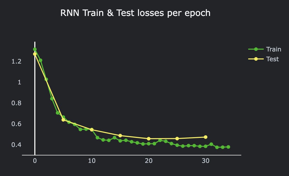
# >>> Train loss: 0.3783
# >>> Val loss: 0.4730
Train & test losses per epoch, RNN model
This model showed 84.3% balanced accuracy on eval dataset. Wow, what a progress!
The major downside to training the RNN model from scratch is that it has to learn the meaning of the words itself – that is the job of the embedding layer. Pre-trained word2vec models are available to use as a ready-made embedding layer, which reduces the number of parameters and adds a lot more meaning to tokens. Let’s use one of the word2vec models available in pytorch – glove, dim=300.
We only need to make minor changes to the Dataset creation – we now want to create a vector of glove pre-defined indexes for each description, and the model architecture.
ds_emb_train = util.PaddedTextVectorDataset(
    data_train["description"],
    data_train["target"],
    emb=glove,
    max_vector_len=max_len,
)
ds_emb_test = util.PaddedTextVectorDataset(
    data_test["description"],
    data_test["target"],
    emb=glove,
    max_vector_len=max_len,
)
dl_emb_train = DataLoader(ds_emb_train, batch_size=512, shuffle=True)
dl_emb_test = DataLoader(ds_emb_test, batch_size=512, shuffle=False)
import torchtext.vocab as vocab
glove = vocab.GloVe(name='6B', dim=300)

class LSTMPretrained(nn.Module):
    def __init__(self, n_hidden, n_out):
        super().__init__()
        self.emb = nn.Embedding.from_pretrained(glove.vectors)
        self.emb.requires_grad_ = False
        self.embedding_dim = 300

        self.n_hidden = n_hidden
        self.n_out = n_out

        self.lstm = nn.LSTM(self.embedding_dim, self.n_hidden, num_layers=1)
        self.dropout = nn.Dropout(0.5)
        self.out = nn.Linear(self.n_hidden, self.n_out)

    def forward(self, sequence, lengths):
        batch_size = sequence.size(1)
        self.hidden = self.init_hidden(batch_size)
        embs = self.emb(sequence)
        embs = pack_padded_sequence(embs, lengths, enforce_sorted=True)
        lstm_out, (self.hidden, _) = self.lstm(embs)
        lstm_out, lengths = pad_packed_sequence(lstm_out)
        dropout = self.dropout(self.hidden[-1])
        output = self.out(dropout)
        return F.log_softmax(output, dim=-1)

    def init_hidden(self, batch_size):
        return Variable(torch.zeros((1, batch_size, self.n_hidden)))
And we’re ready to train!
n_hidden = 50
n_out = len(label_2_idx)

emb_model = LSTMPretrained(n_hidden, n_out)
opt = optim.Adam(emb_model.parameters(), 1e-2)

util.fit(model=emb_model, train_dl=dl_emb_train, test_dl=dl_emb_test,
         loss_fn=F.cross_entropy, opt=opt, epochs=11)
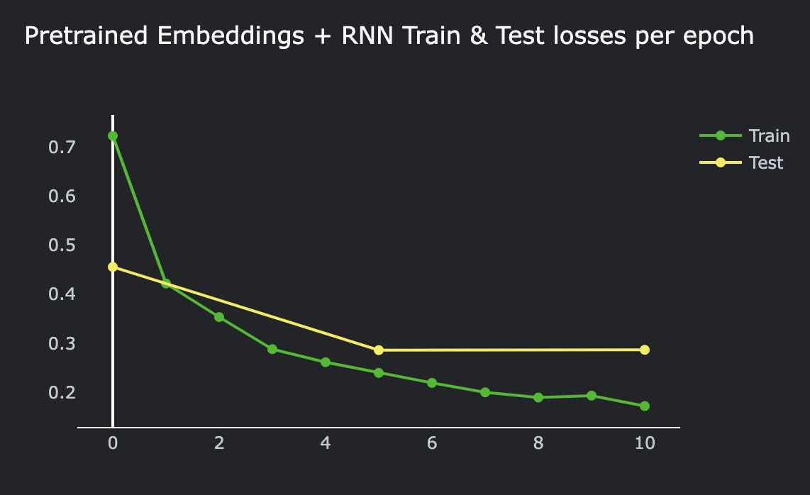
Train & test losses per epoch, RNN model + pre-trained embeddings
Now we’re getting 93.7% balanced accuracy on eval dataset. Woo!
Modern state-of-the-art models for working with sequences are transformers. However, to train a transformer from scratch, we would need massive amounts of data and computational resources. What we can try here – is to fine-tune one of the pre-trained models to serve our purpose. To do this we need to download a pre-trained BERT modeland add dropout and linear layer to get the final prediction. It’s recommended to train a tuned model for 4 epochs. I trained only 2 extra epochs to save time – it took me 40 minutes to do that.
from transformers import BertModel

class BERTModel(nn.Module):
    def __init__(self, n_out=12):
        super(BERTModel, self).__init__()
        self.l1 = BertModel.from_pretrained('bert-base-uncased')
        self.l2 = nn.Dropout(0.3)
        self.l3 = nn.Linear(768, n_out)


    def forward(self, ids, mask, token_type_ids):
        output_1 = self.l1(ids, attention_mask = mask, token_type_ids = token_type_ids)
        output_2 = self.l2(output_1.pooler_output)
        output = self.l3(output_2)
        return output
ds_train_bert = bert.get_dataset(
    list(data_train["description"]),
    list(data_train["target"]),
    max_vector_len=64
)
ds_test_bert = bert.get_dataset(
    list(data_test["description"]),
    list(data_test["target"]),
    max_vector_len=64
)

dl_train_bert = DataLoader(ds_train_bert, sampler=RandomSampler(ds_train_bert), batch_size=batch_size)
dl_test_bert = DataLoader(ds_test_bert, sampler=SequentialSampler(ds_test_bert), batch_size=batch_size)
b_model = bert.BERTModel(n_out=4)
b_model.to(torch.device("cpu"))

def loss_fn(outputs, targets):
    return torch.nn.BCEWithLogitsLoss()(outputs, targets)

optimizer = optim.AdamW(b_model.parameters(), lr=2e-5, eps=1e-8)
epochs = 2
scheduler = get_linear_schedule_with_warmup(
    optimizer,
    num_warmup_steps=0,
    num_training_steps=total_steps
)

bert.fit(b_model, dl_train_bert, dl_test_bert, optimizer, scheduler, loss_fn, device, epochs=epochs)
torch.save(b_model, "models/bert_fine_tuned")
Training log:
2024-02-29 19:38:13.383953	Epoch 1 / 2
Training...
2024-02-29 19:40:39.303002	step 40 / 305 done
2024-02-29 19:43:04.482043	step 80 / 305 done
2024-02-29 19:45:27.767488	step 120 / 305 done
2024-02-29 19:47:53.156420	step 160 / 305 done
2024-02-29 19:50:20.117272	step 200 / 305 done
2024-02-29 19:52:47.988203	step 240 / 305 done
2024-02-29 19:55:16.812437	step 280 / 305 done
2024-02-29 19:56:46.990367	Average training loss: 0.18

2024-02-29 19:56:46.990932	Validating...
2024-02-29 19:57:51.182859	Average validation loss: 0.10

2024-02-29 19:57:51.182948	Epoch 2 / 2
Training...
2024-02-29 20:00:25.110818	step 40 / 305 done
2024-02-29 20:02:56.240693	step 80 / 305 done
2024-02-29 20:05:25.647311	step 120 / 305 done
2024-02-29 20:07:53.668489	step 160 / 305 done
2024-02-29 20:10:33.936778	step 200 / 305 done
2024-02-29 20:13:03.217450	step 240 / 305 done
2024-02-29 20:15:28.384958	step 280 / 305 done
2024-02-29 20:16:57.004078	Average training loss: 0.08

2024-02-29 20:16:57.004657	Validating...
2024-02-29 20:18:01.546235	Average validation loss: 0.09
Finally, fine tuned BERT model shows whopping 95.1% balanced accuracy on eval dataset.
We’ve already established a list of considerations to look at to make a final well-informed choice.
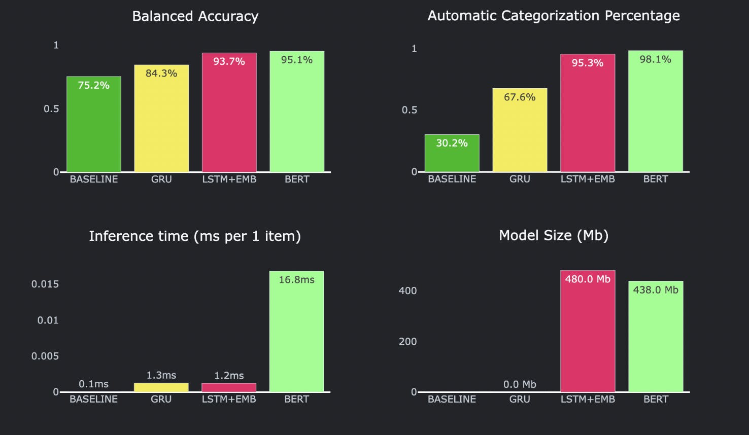
Here are charts showing measurable parameters:
Models’ performance metrics
Although fine-tuned BERT is leading in quality, RNN with pre-trained embedding layer LSTM+EMB is a close second, only falling behind by 3% of automatic category assignments.
On the other hand, the inference time of fine-tuned BERT is 14 times longer than LSTM+EMB. This will add up in backend maintenance costs which will probably outweigh the benefits fine-tuned BERT brings over LSTM+EMB.
As for interoperability, our baseline logistic regression model is by far the most interpretable and any neural network loses to it in this regard. At the same time, the baseline is probably the least scalable – adding categories will decrease the already low quality of the baseline.
Even though BERT seems like the superstar with its high accuracy, we end up going with the RNN with a pre-trained embedding layer. Why? It’s pretty accurate, not too slow, and doesn’t get too complicated to handle when things get big.
Hope you enjoyed this case study. Which model would you have chosen and why?
This article was originally published by Maria K on HackerNoon.
Interest in the apartment industry is reaching fever pitch as author Chris Schembra, mogul Barbara…
Let’s take a closer look at ‘Browsergate’: is LinkedIn really running the biggest corporate espionage…
Valencia’s tech ecosystem is getting a big win this June 12-14 as Techstars Startup Weekend announces…
In the upper floors of corporate America, budgets are larger than ever, board presentations are…
If your content is deemed to be disinformation by the ministry of truth, your speech…
In the latest episode of Brains Byte Back, host Erick Espinosa sits down with Dr.…